Oftentimes, we are faced with the challenge of making decisions without the amount of information we would like to have. In many of those occasions, the decision we make has a tremendous impact on aspects such as safety or cost, and it has been selected by us using some proxy of the real information we really needed. This is the case with off-the-shelf component selection for our systems, in which many times the deciding factor tends to be a few cents difference in unit price, for components that will be used thousands and thousands of times over the manufacturing life of our product. As many will know by now, the price tag of a component is just a fraction of the total cost of that component for us, and it shouldn't be trusted as the sole source of truth to make such an important decision. We'll see in this article how to add another dimension to our decision tree in terms of reliability, so that we can make data-driven choices.

Component face-off

In this example, we need to select an endstop microswitch, of which seven units shall be integrated into our system for actuation control purposes. We are expecting to sell a significant amount of these systems per year, so the unit price of the selected switch will be an important factor to take into account when choosing it. That, and other technical specifications like operating voltage, current, connector typology, and physical dimensions, amongst others, have limited our contender list to two options from two different manufacturers:

• Option A:
  • Price: 1.59€
  • Expected life (electrical): 50,000 cycles
  • Expected life (mechanical): 1,000,000 cycles
  • Max. operating frequency: 30 operations/minute
• Option B:
  • Price: 1.83€
  • Expected life (electrical): 50,000 cycles
  • Expected life (mechanical): 1,500,000 cycles
  • Max. operating frequency: N/A

As seen in these specifications, some manufacturers add the expected life values of their products to their brochures as it can be very relevant for their customers. However, a single number of hours can be of little use in many cases. The price difference is evidently a deciding factor in cases like this where everything else is tied, but as mentioned before, it may not be the best answer to our problem. In terms of mechanical reliability, Option B seems the obvious choice for our system, but we also see that the electrical reliability of these switches is the limiting factor, which makes the mechanical durability less relevant.

We, being very analytical and willing to dig a bit deeper, decide to run a test to get more information about our contenders.

Setting up the test

Some back of the envelope calculations tell us that with the limiting operating frequency of Option A, we could perform a test that actuates the switch 30 times per minute, or the equivalent of 43,200 times per day. Given the expected electrical life claimed by the manufacturer, this stress test conditions will take around a day to have each switch reach their failure point.

We decide to design an ad hoc PCB that consists of the tested microswitch and a tiny display that will show the times the switch has been pushed. An actuation system can push all the switches collectively at the testing frequency described above.

If we fabricate 10 of these ad hoc PCBs, we’ll have about 10 failed switches every day or day and a half. By replacing the failed switches with new ones, and putting them back in the test, we can easily have around 60 or 70 failed switches for a test that takes less than two weeks to complete. Having 30 to 35 units of each option seems sufficient to get good results about them (and we could always run the test for a few more days if we’re not satisfied with the precision of the results).

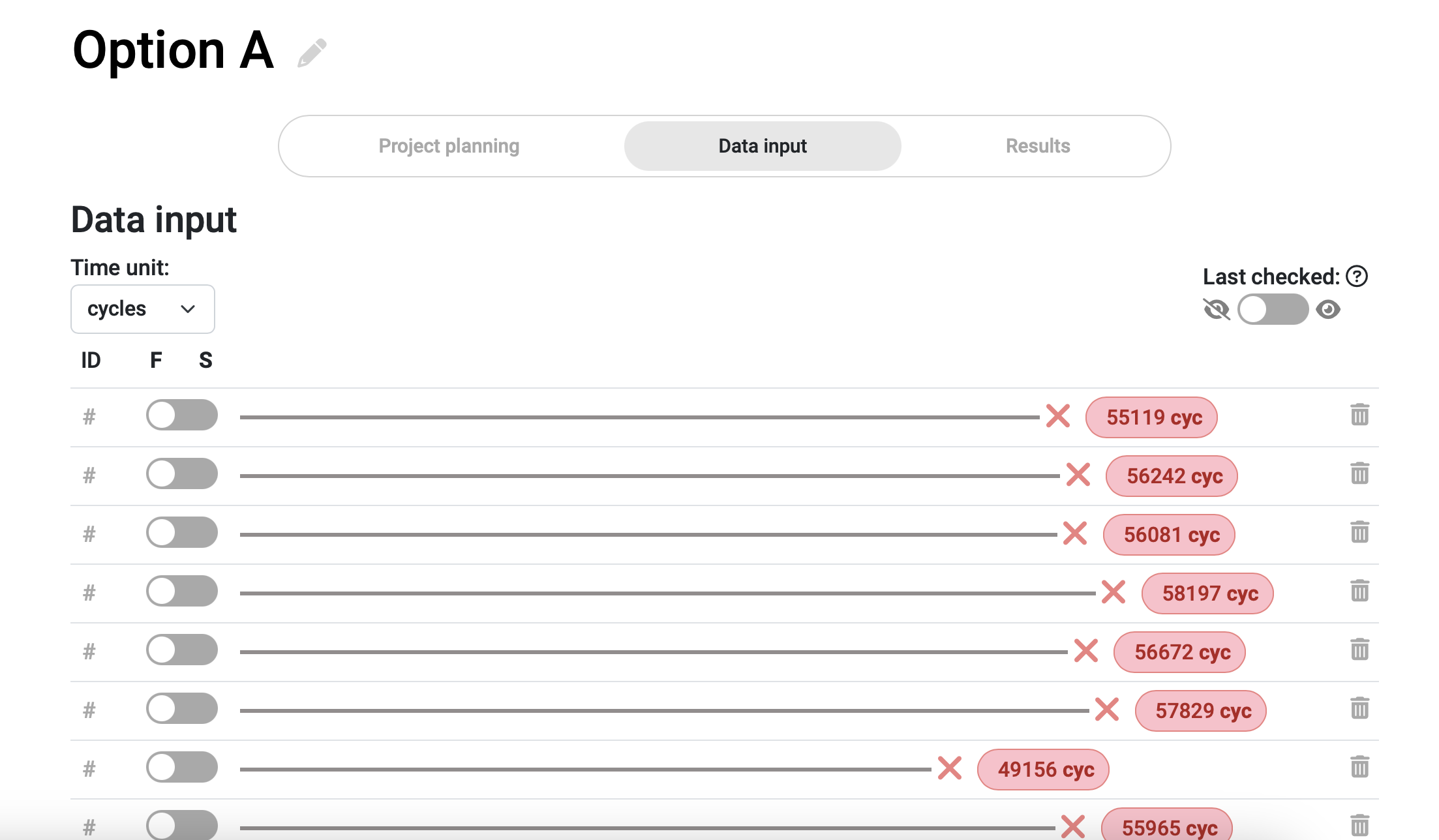
Because we added displays that increase the count every time the switch is pushed, by the time it fails (presumably being unable to either open or close the circuit), our counter will stop adding up and the exact amount of cycles before failure will be registered. This data input in our Broadstat project will look somewhat like this:

Results

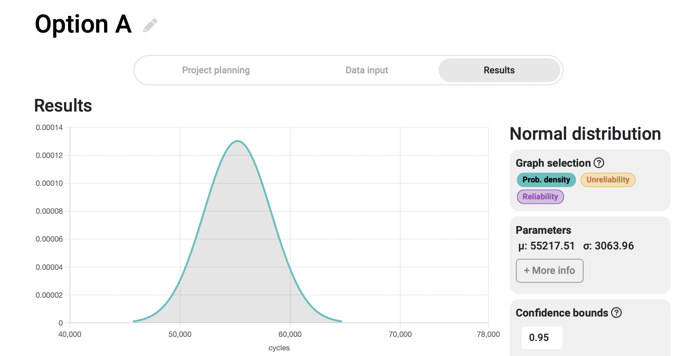
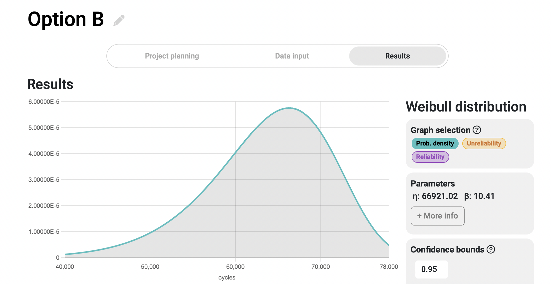
Once we input the data for the two options in two different Broadstat projects, we can click on the results tab to automatically calculate the statistical distribution of each of them. Upon first glance, we can observe significant differences between their respective probability density functions.

For comparison purposes, the x-axis of both graphs has been equalized, making it easier to see the differences in time between the two systems. As can be seen, the failure probability curve of Option A is sharper and narrower, indicating that the failures occur within a shorter time span compared to the Option B curve.

By creating Highlighted datapoints in our Broadstat projects and asking for specific results at a certain number of cycles, we can obtain more detailed information. For the question "What is the probability of reaching 50,000 cycles?" for each option, the responses are as follows:

• Option A: The probability that this system remains functional until reaching 50,000.00 cycles of operation is 96%, with the minimum and maximum values of this probability being 88% and 99%, respectively.
• Option B: The probability that this system remains functional until reaching 50,000.00 cycles of operation is 95%, with the minimum and maximum values of this probability being 88% and 98%, respectively.

Therefore, we can accept that both manufacturers' claims are more or less acceptable, and there is a high probability that 50,000 cycles can be achieved by both switches. We also observe that the precision range of the responses in this particular section of the graph is within a 10% margin of probability (from 88% to 98% for Option B's example). If we are not satisfied with this 10% margin, we can continue the test for a few more days to obtain more precise results.

However, we did not set up this study simply to corroborate the manufacturers' reliability claims, but to obtain a more detailed set of results regarding these components' expected behavior. So let's see how this could be interpreted depending on what we need for our system.

Scenario #1

In this scenario, let’s assume that given the expected level of usage of this system and the lifespan we set for it in our requirements, our target number of cycles to reach is 45,000. Once this value is reached, we consider the system to have reached the end of its life. If we check this value the same way we did previously for the 50,000 cycles, we obtain the following:

• Option A: the probability of reaching 45,000 cycles is 100% (99% for the conservative estimate)
• Option B: the probability of reaching 45,000 cycles is 98% (94% for the conservative estimate; 100% for the optimistic one)

Given these results and adding the fact that Option A is cheaper, we have a clear winner.

Scenario #2

We expect a small fraction of our userbase to operate their systems significantly more than the average user. These are really dedicated users that embrace our brand better than the rest, and we especially don’t want to let them down. Their estimated usage of this system over its lifetime is around 60,000 cycles. However, we don’t want to oversize our product to ensure this value for everyone, considering that this intensity of use will only be related to a small population of users. Let’s see how it will do for both options:

• Option A: the probability of reaching 60,000 cycles is 6% (2% for the conservative estimate; 15% for the optimistic one)
• Option B: the probability of reaching 60,000 cycles is 73% (58% for the conservative estimate; 83% for the optimistic one)

As you can see, the difference here is huge! Because the probability of failure curve for Option A is so compact, it concentrates most of the failures around 55,000 cycles and the probability of reaching our target value is very small. If this were a determining factor, Option B should be the selected component.

Scenario #3

Now imagine that instead of using seven units of a component that’s under 2€, we are discussing the selection of a subsystem that’s used in the device and represents 20% of the cost of production of our product. Not only that, but the supply chain is relatively complex, so it takes several weeks for us to obtain it. We are also imagining in this scenario that the desired lifetime of our system is longer than before, which will entail the need for one or two replacements of this expensive component over its whole usage period.

Having that in mind, and thinking about our customers, who can’t have more than a day of downtime, we need to make a decision that guarantees we are always ready to pick up a replacement from our warehouse and install it at their premises as fast as possible. To address this, we have two alternatives:

• Alternative 1: store always a significant amount of spares in your warehouse so that you can guarantee you’ll be able to respond whenever it’s necessary. These replacements will be paid by the costumer whenever you install them, but you’ll probably be occupying more precious storage space than necessary, and the rotation of these goods will be really slow, which means your cashflow cycle gets worsened.
• Alternative 2: you monitor the usage of your customers’ systems (with their knowledge, obviously) and make an estimation of when they are going to need the replacement. Once you’ve done this prediction, you can order the spares in advance so that you’re ready for when the time comes. This doesn’t mean that you can’t hold a bit of extra stock for any unexpected events, but it wouldn’t be as significative as in the first alternative.

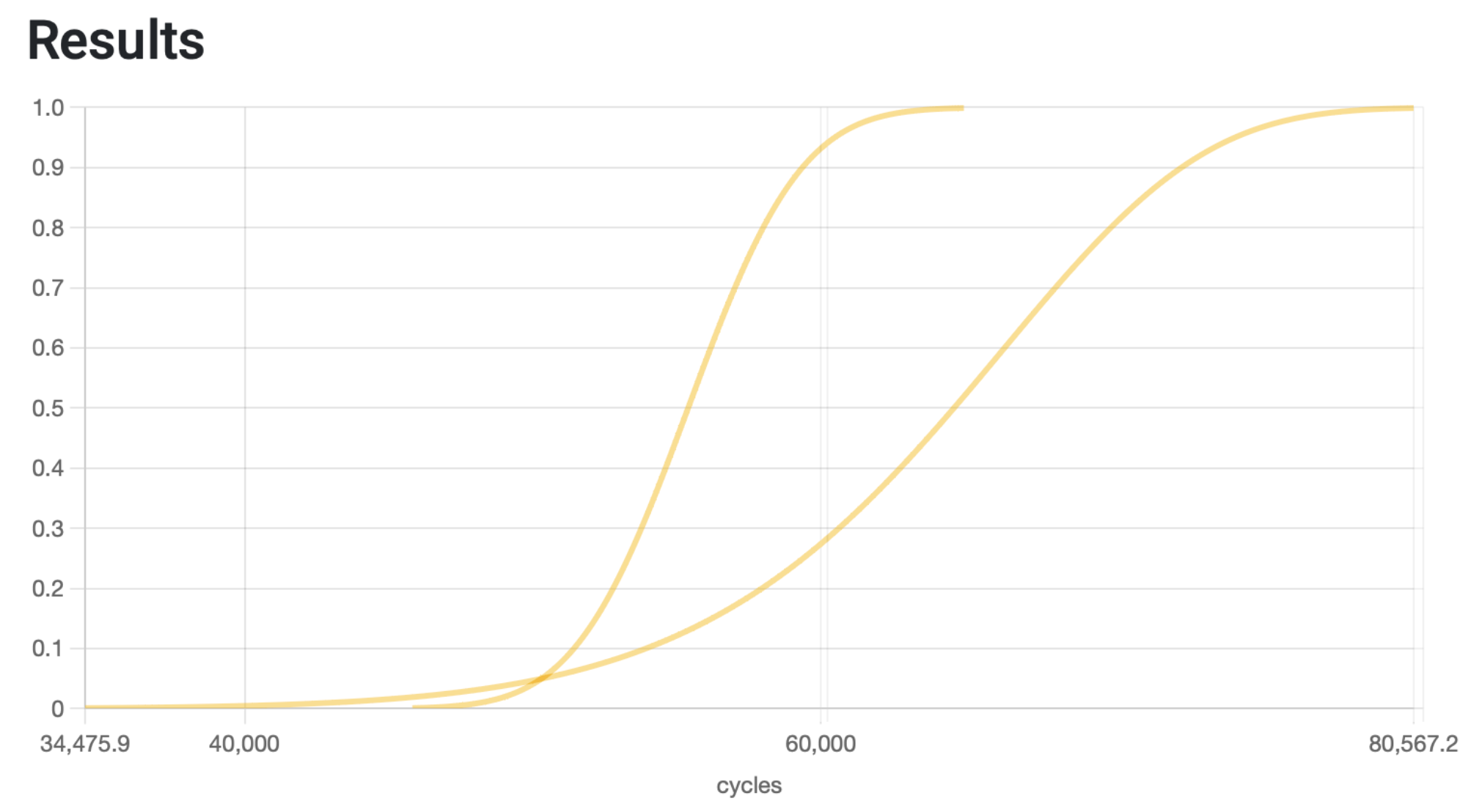
As you may imagine, the second alternative is a more lean approach to stock management, which let’s you allocate your resources somewhere else. However, if we go back to our two graphs of probability of failure, they are not equally suitable for this approach: the subsystem with Option A’s curve has a more compact timeframe in which the failure for a specific device is expected to happen, while for Option B the occurrence probability spreads over a longer period. Regardless of the usage frequency of our customers, we can statistically say that we may hold the stock more than twice as much time in our warehouse if we choose Option B over Option A. This is because the period it takes Option B to go from 0% probability of failure to 100% is more than double what it does for Option A. If we overlap both unreliability curves, this becomes clearer.

Conclusion

There is no exact number of cycles or hours of usage that can definitively determine the better selection for us in terms of reliability. It is more closely tied to distribution shapes, values at a specific moment of use, and how these factors impact not only our designs but also the entire product lifecycle and its economics. Choosing the best alternatives requires critical thinking, a deep understanding of our company's needs and the services we provide to our customers, and the ability to extrapolate this knowledge for informed decision-making.