Even when we put our deepest care into the manufacturing of our products, we are always subject to potential flaws or defects that may be hard to detect and can jeopardize their quality. That’s why the job of the Quality Assurance department is so important—to guarantee that these products maintain certain levels of performance, reliability, appearance, etc. However, some reductions in the quality of a component or subsystem can’t be perceived until it’s too late, and then reactive measures need to be taken: recalls for a specific lot of production, an increase in service calls, refunds… It’s not pretty, and it not only costs a lot of money but also damages our brand image.

As an illustrative example, a slight variation in the mold release additive mixed with the raw polymer before a plastic injection process can be sufficient to completely change the durability of a part. When a part from this "cursed" batch arrives from our injection supplier, it looks exactly the same as a good one, and even some of our standardized quality tests yield equivalent results, like break resistance tests and so on. So it can be the case that, even when using the base material and injection conditions you approved during the homologation phase, this part no longer fulfills the necessary technical specifications, and, to make matters worse, it goes undetected.

Burn-in tests

It is a common practice to perform burn-in tests during production, which consist of submitting a finished unit to a certain number of cycles of usage to detect defective components and early failures before the unit is shipped to its purchaser. These cycles are non-destructive and typically cover a few days of operation, allowing the detection of many cases of sub-standard quality that may occur during the production and initial usage of the product. However, burn-in tests can’t detect quality issues related to extended usage that may appear further down the line. For example, for a component that’s supposed to work reliably for 1000 days, a failure that occurs after 300 days of operation is a quality catastrophe that won’t be detected in a burn-in test lasting 72 hours.

Reliability characterization

If our aim is to evaluate the quality of our system in terms of reliability, the first thing we need to do is understand its reliability behavior in normal circumstances. Thanks to Broadstat, that has never been easier.

Imagine we want to test a subsystem that cycles 500 times a day under normal operating conditions and sits idle the rest of the time. In our lab test, we can choose to perform our stress cycling at that same rate, or we can actuate this subsystem without stopping between cycles, allowing us to fit 16,000 actuations in a single day (this hypothetical cycle lasts 5.4 seconds to complete). If we divide both frequency-of-use numbers, we come up with a factor of x32, known as a Usage Ratio Acceleration factor. This factor is very useful because we don’t interfere with the operating conditions of our subsystem to accelerate our results; we simply make better use of our time. By performing our test this way, we’ll have to wait 32 times less time to obtain failure data.

Let’s assume we set up the mentioned test and submit 25 sample units to it, which, after a few weeks of unstopped actuation, reach their failure points. As an example, one of the units fails after 57 days of the test, which in real life is equivalent to 1,824 days (remember the x32 factor). We can input our information into our Broadstat project as 1,824 days or as 912,000 cycles, whichever we prefer, as long as we stay consistent with the rest of the values of the test.

After introducing all the 25 failure data values to the project, the automatically calculated results look like this:

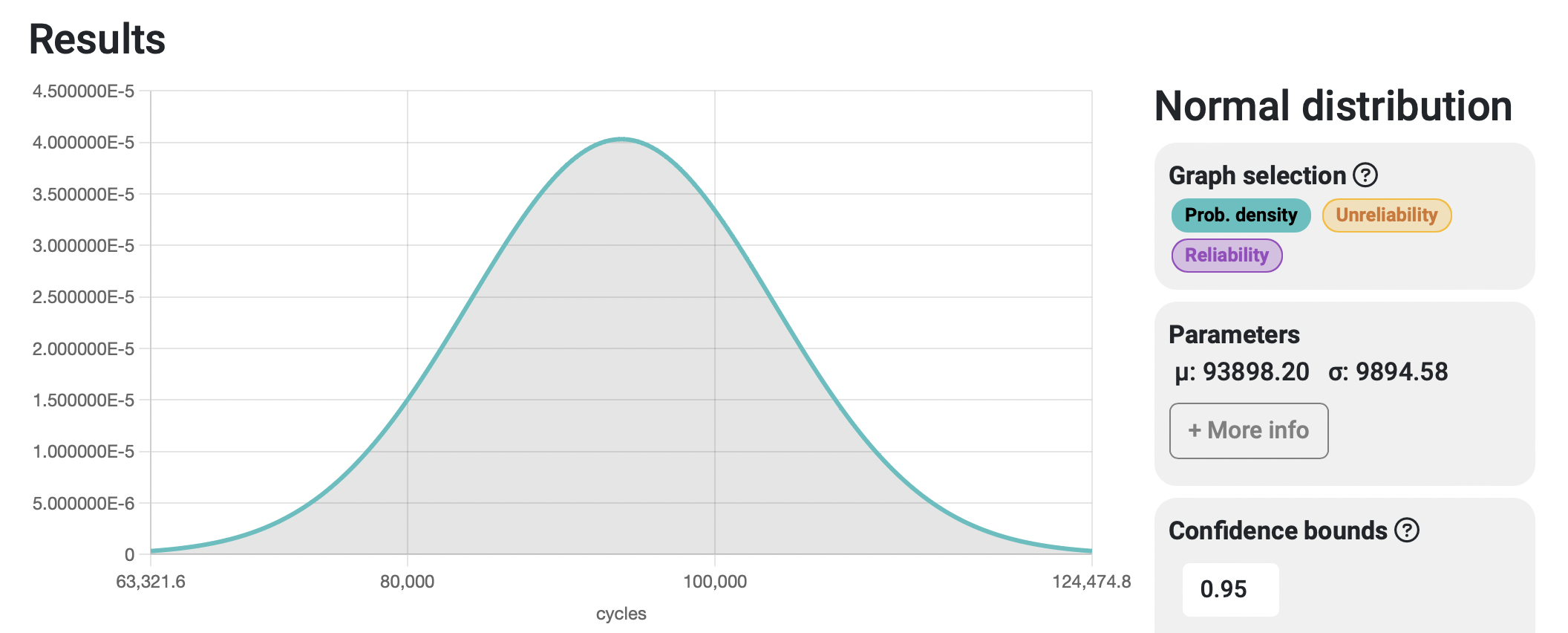
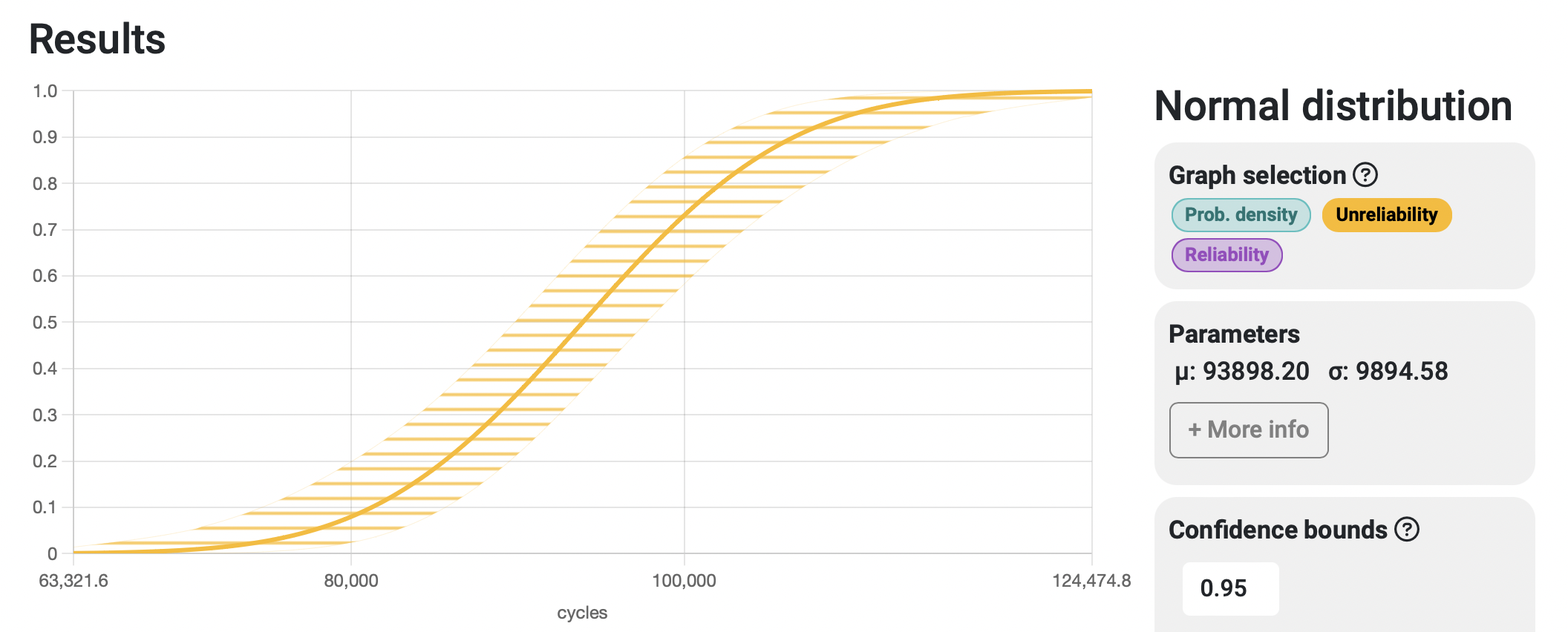
The green curve shows the failure probability density function, or how probable it is to experience a failure at a specific point in time. The yellow curve, or unreliability function, shows the accumulated probability of failure over time, with a 0% chance of failure at the left end of the curve and a 100% chance at the right end.

We have successfully characterized the failure behavior of our system and are ready to use it to our advantage to make better-informed decisions.

Setting our threshold limits

If you were to analyze a production sample and determine whether it follows the usual failure behavior of your reference system or not, what would be the threshold value you would choose in terms of reliability? Let’s rephrase the question: in our ongoing example, if our production sample were to fail after 100,000 cycles of stress, would you say it’s within the normal range of values for failure in our system? What about 70,000 cycles?

A common value for cases like this is the one at which the probability of failure is 5%. Some people prefer to use a value of 1%, or something in between, but the idea is that it has to be a fairly small value that can tell us that something is off. If we choose the 5% threshold, we can request the unreliability value of our system using Broadstat’s Highlighted points.

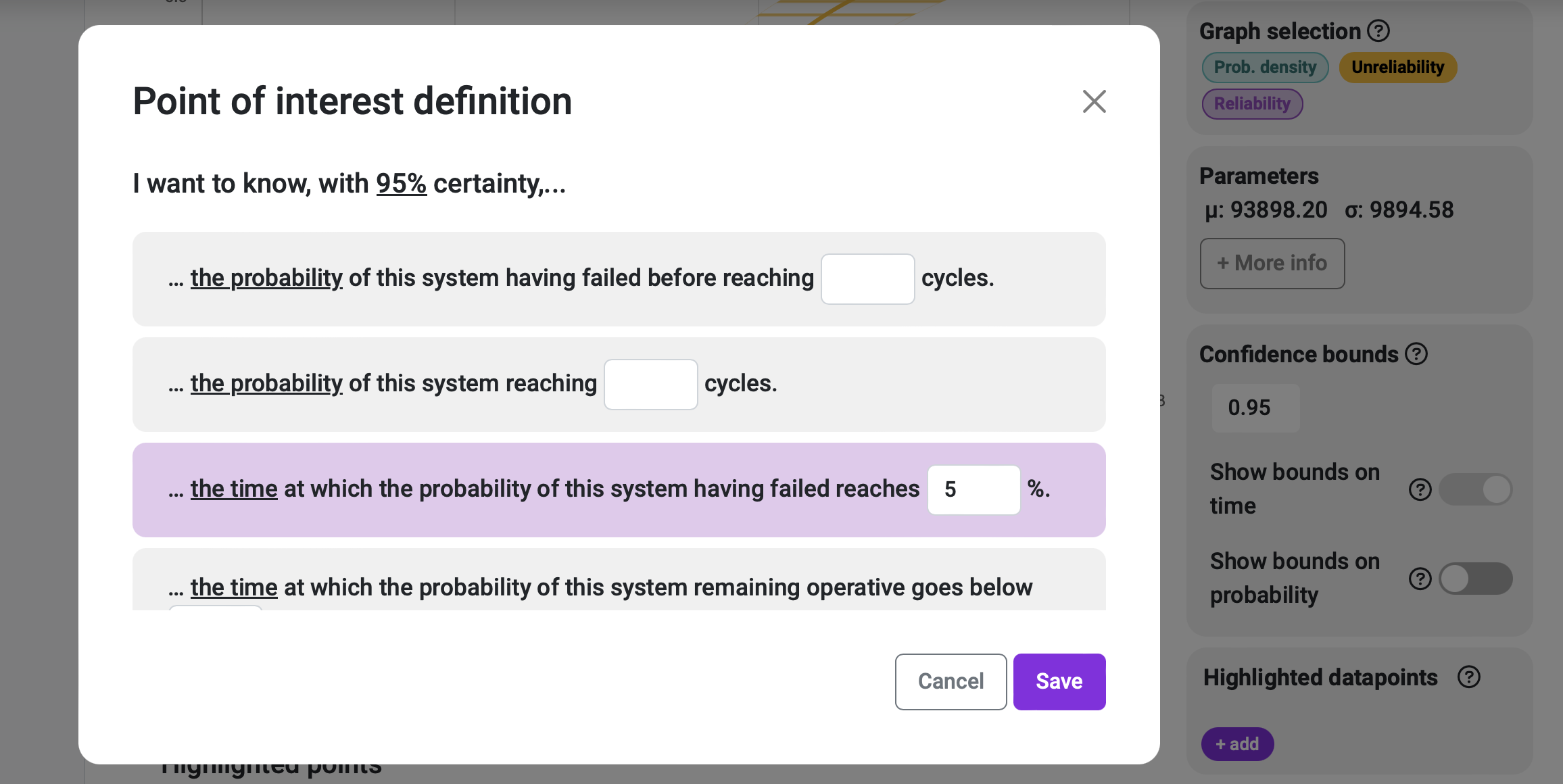
The response to this Highlighted point is the following:

• The system has a 5% probability of not reaching 77623.06 cycles of operation. This value, known as an unreliability of 5%, is estimated to occur between 70395.08 and 82711.45 cycles when accounting for confidence variability.

It is displayed in the graph section as well, as seen below.

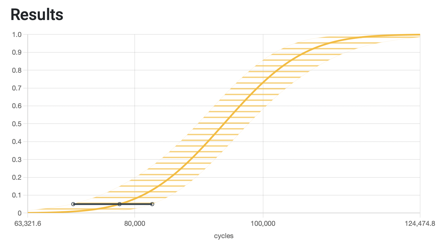
This informs us that our nominal curve reaches a 5% accumulated probability of failure at 77,623 cycles, while the conservative estimation places this value at 70,395 cycles.

Evaluating production samples

Now that we have characterized our system in its standard operating behavior and have selected our threshold value to classify parameters as outliers, the only thing left is implementing it in our production process and starting testing samples from whatever batches we want to analyze.

If you think about the 5% failure probability, it means that 1 out of every 20 samples we test should fail when reaching the number of cycles shown before, which actually is not such an improbable thing to happen after all. Simply testing one unit of a batch and claiming the whole production is faulty just because it was below the 5% margin would be a mistake. For that reason, we should test a few units per batch so that we can differentiate between real production outliers and normal low-tailed cases.

An interesting approach would be to extract 3 or 5 units out of our batch and run our cycling test on them. If all of them pass our minimum threshold barrier of 70,395 cycles (if we want to use the conservative estimation values), we may declare the batch as normal. If one of them fails to reach it but the others do, there’s probably nothing to worry about. However, if multiple units or even all of them fail to reach our threshold number of cycles, we may probably be dealing with a defective lot.

Performing test acceleration

If you liked what you’ve just read but thought, “Well, there’s no way I can implement this because my production throughput is way shorter than the testing time, and I can’t hold my products until the study tells me it’s OK to ship them,” there may be some good news for you. Typically, systems’ reliability reacts to the environment and the operating conditions they’re under and can be shortened by increasing parameters like ambient temperature or voltage.

Let’s say we have characterized our system as we saw in the previous paragraphs, and it has validated our reliability requirements for use in normal operating conditions. However, we can't wait five weeks for each test to finish if we want to implement faulty batch detection techniques during the production life of our system. We could then make a second characterization of our system under non-normal operating conditions, which can take way less time to finish, and use that as our benchmark to compare against for our production quality tests (also run under the same non-normal conditions).

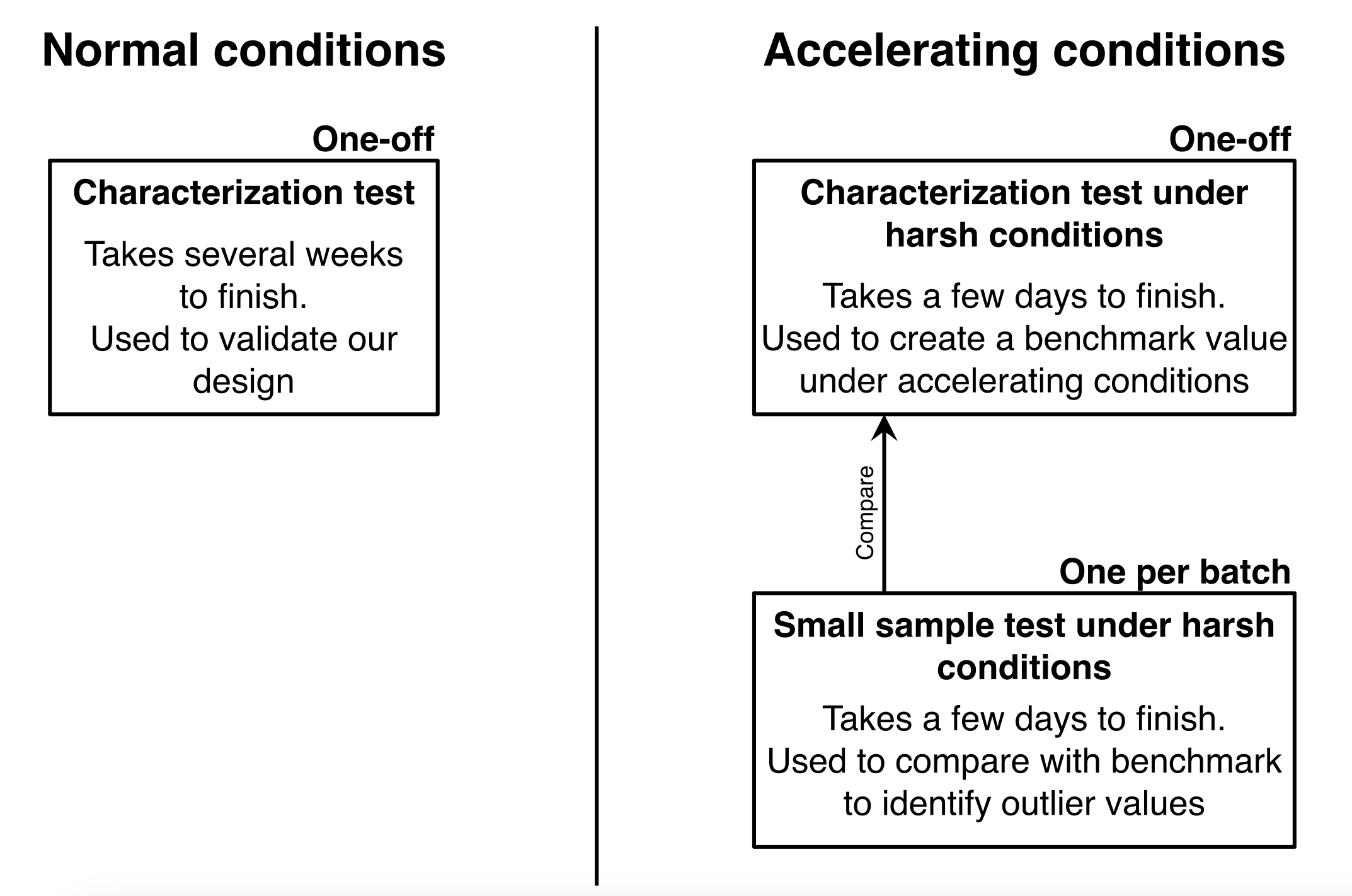
As long as we compare oranges to oranges, and the checks remain relative to each other by using the same accelerated environment, we can speed up our tests without worries. Some of the parameters that are known to accelerate failures are:

• Temperature (constant or cycled)
• Voltage, current (constant or cycled)
• Mechanical stress
• Humidity
• Vibration
• Chemical atmosphere

So, in this case, a sample that would normally take 5 weeks of constant cycling to fail under normal operating conditions may only take a few days when the ambient temperature of the test lab/chamber and the system voltage are raised to a certain degree. You can combine the acceleration factors at will, but there is one rule that can never be broken:

If you are testing a system in which the evaluated failure mode is a belt that breaks, and due to an increase in humidity of your test chamber, the stepper motors are the faulty component of the system, you have activated a failure mode that wasn’t relevant in normal operating conditions. It also wouldn’t be acceptable if the belts normally break, and your accelerated test dissolves them in some acid because the failure mode would be different.

Conclusion

It is within our reach to test our finished products or inbound components for flaws related to reliability, so that we can minimize unexpected issues that can highly deteriorate our brand image. As with many other important things in life, it requires patience and discipline to implement processes like those discussed in this article, but these are also the practices that separate mid-tier companies from the ones at the very top. Luckily, a tool like Broadstat can facilitate the application of checks like these, bringing you one step closer to achieving excellence in what you do.